


POLLUTE - 污染物运移分析软件
POLLUTE是一款污染物运移分析软件。POLLUTE被广泛用于垃圾填埋设计和环境补救领域,可将 1.5 维度的解决方案运用到对流 - 扩散方程中。与有限元和有限差方程不同的是,POLLUTE要时间推进步骤,因此降低了计算工作量,减少数值不稳定问题的产生。
POLLUTE在工业领域已有15年以上的应用,它是一种经测试的污染物迁移分析程序,已广泛用于垃圾掩埋场设计和修复中 。可以考虑的垃圾填埋场设计范围,从天然粘性含水层上的系统到复合衬垫、多重屏障和多重含水层。
主要:
1、非线性吸附作用;
2、反射性和生物过程的腐烂;
3、通过断面的传输;
4、被动沉降,相变;
5、随时间变化的。
可以使用程序向导或通过选择预先创建的模型中的来从头开始创建模型:例如,主衬垫填埋场和次衬垫填埋场。垂直迁移和水平迁移。
污染数据输入
使用屏幕顶部的主菜单栏,可以创建,编辑和执行数据集。然后可以显示和打印这些数据集的输出。
可以使用数据菜单创建或编辑POLLUTE数据集。数据集由常规矿床数据,地层数据,边界条件和可选的功能组成。
输入有关模型的数据,例如:
数据集标题
土壤层数(每层可以具有不同的属性)
穿过土壤层的速度
拉普拉斯转换参数(默认值通常就足够了)
污染层数据
对于层,可以指定以下内容:
子层数
厚度
干密度
水动力弥散系数
分配系数
骨折类型(如果存在)
创建层都可能破裂。这些裂缝可以是一维,二维或三维的。在裂缝层中,该程序沿裂缝的对流 - 弥散运移,并扩散到裂痕两侧的基质中。
污染边界条件
数据集都有两个边界,在边界层的顶部,在层的底部。顶部边界通常是与污染源(有限质量或恒定浓度)的接触点,底部边界通常是与含水层(固定流出)或基岩(零流量)的接触点。
有限质量边界条件
有限质量边界条件可用于表示污染源,例如垃圾填埋场。如果污染物的质量是有限的,则随着污染质量被输送到下面的层中或被渗滤液收集系统请去除,污染源出的污染浓度将下降。
固定流程速度边界条件
此边界条件可用于表示数据集中各层下方的含水层。随着质量从上方格层传输到含水层中,然后通过基础层中的水平速度传输出去,该含水层中的浓度将随时间变化。
污染
除了基本数据参数以外,模型中还可以使用功能。可以从多向选择菜单中选择这些功能中的一项或多项。
放射性/生物
衰变可以对放射性或生物衰变进行建模。通过制定源,层和基础含水层的半衰期来考虑一阶衰变。这些层可以具有相同的半衰期,后者可以将半衰期指定为深度的函数。
深度间隔浓度分布图
为了模拟各层中的背景弄丢,可以使用初始浓度分布图。使用此选项,可以将层中的初始浓度指定为深度的函数。此外,可以在模型开始时指定流入土壤和Polar region 的通量。
Freundlich和Langmuir非线性吸附
可以考虑Freundlich或Langmuri非线性吸附。使用非线性吸附时,该程序将各层分成子层,并使用迭代技术确定子层的等效线性分布系数。
组内的属性增量
此选项用于随着时间改变模型的属性。用户可以改变源浓度,污染物质量,手机的渗滤液量,达西速度,分散度和含水层速度。例如,该选项可用于模拟垃圾填埋场渗滤液收集系统的渐进式破坏。时间分为几组。在组中,属性可以随时间恒定或可以随时间线性增加。可以指定细节开始源中的浓度
被动接收器
模型中可以使用被动接收器。被动水槽是水平速度所在的一层。这将具有去除污染物的作用。通常,无元水槽用于表示次要渗滤液收集系统或多个含水层。
蒙特卡洛变量输入法
蒙特卡洛模拟可用于评估某些模型数据的不确定性的影响。使用这种方法,使用概率分布描述比确定的数据值。经过无数次模拟后将生成深度处污染物峰值浓度的 概率分布。
主衬板(字幕D)垃圾填埋场
有一些选项创建和自定义预定义的模型。这些模型带有主要渗滤液收集场和复合衬里的垃圾填埋场
主要和辅助陈丽垃圾填埋场
有多种选项创建和定制预定义的模型。这些模型具有主要渗滤液手机和复合衬里的垃圾填埋场和具有主要和次要渗滤液收集和复合衬里的垃圾填埋场。这些填埋场输入选项中,在层名称选择“是”或“否”,就可以选择分类到土工膜,粘土衬里。
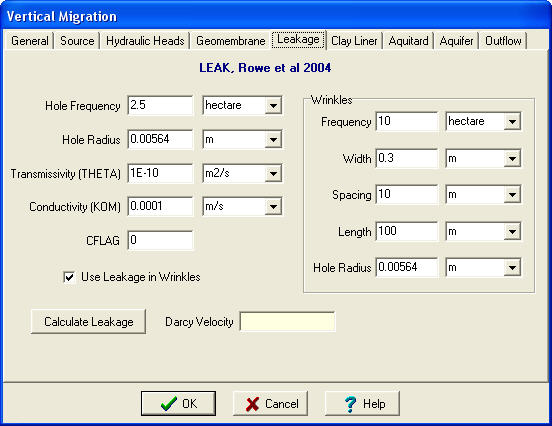
土工模孔数据
土工膜与黏土衬层之间的接触类型外,“泄露量”还取决于裂缝类型,大小和频率。
有限质量源
垃圾填埋场的污染源可以是有限质量的,也可以是恒定浓度的。如果源类型为有限质量,则可以指定污染物的废物厚度和密度,通过盖子的渗透和相关数据。
主黏土衬里或GCL
对于模型中存在的层,可以单位指定参数。改成将自动将单位转换为SI或US。衬垫可以是黏土或土工合成黏土衬垫。
含水层
如果垃圾填埋场下方存在含水层,则可以指定含水层厚度和孔隙率。该程序将自动计算含水层中的小流出速度。可以指定此值或以上的值。
污染模型执行
计算浓度
创建数据集后,可执行模型在数量深处计算污染物的浓度,或者选定深度处自动确定较大浓度。从而使其成为检查设计方案和“灵敏度分析”作用。
污染结果输出
执行完模型后,可以显示,图形和打印输出文件。图表可以是浓度对时间,浓度对深度,通量对时间和颜色浓度。这些图形也可以秦松地在几种类型的打印机上打印。图形的默认值是自动确定的。可以更改这些值以允许定制图形。对于浓度与时间。
浓度与时间关系
随时间的变化的浓度图显示了所研究深度的污染物浓度随时间的变化。使用这些图,可以确定深度处的峰浓度。该值也会自动显示在图形的顶部。
浓度与深度
关系浓度与深度的关系图显示了疼时间或所以计算时间的污染物浓度随深度的变化。
通量与时间的关系可以绘制出随时间推移进入土壤层顶部和流出土壤层底部的总通量。
颜色浓度图
浓度随时间和深度的变化图可用于说明污染物羽流随时间向更深的深度移动。
打印选项
图形可以在显示时按“P”键进行打印。可以控制打印图形的功能,例如大小,标题和字体。
污染工具
可使用工具来帮助创建和检查数据集
计算器
计算器工具,用于确定达西速度和污染物质量
帮助
可以按F1键访问上下文相关的帮助文本。显示的信息可交叉引用,通过单击突出显示的文本来提示他们。
功能:
POLLUTE程序使模型的创建,编辑,执行,打印和显示,可以使用程序向导或通过选择预先创建的模型之一从头开始创建模型。
POLLUTE基于数据存储的项目概念,其中用户拥有项目库,并且在项目中都有模型。使用此方法,Microsoft Access 2000数据库用于存储项目。项目都存储在目录中,该目录可以位于同一台计算机上,也可以分布在整个网络中。主数据库用于跟踪项目位置,主项目数据库还用于存储项目中的数据(例如符号库)。
以下功能项目的创建和编辑:
-
存储在Access 2000数据库中的项目
-
项目数量
-
可以创建新项目
-
项目目录是自动创建
-
可以删除项目目录
-
可以导入计算机上的项目
-
项目可以导出到计算机
-
可以自动备份项目
-
备份的项目可以还原
-
程序版本6中的模型数据可以导入到项目中
模型用于表示地下岩性,围绕系统和要研究的污染物源。这些模型可用于研究垃圾填埋场,掩埋垃圾,溢出物,泄湖,屏障系统等的影响。研究区域应分组为项目。项目用于在研究区域中存储模型。创建模型后,可以运行该模型以计算指定深度和时间的污染物浓度。
POLLUTE的一些功能:
-
使用空白模型,向导或输入模型可以创建新模型。
-
模型的图形图在创建时显示
-
模型200个图层创建层可1,2或3维裂缝
-
可以为层指定扩散系数,分配系数和相变参数
-
顶部边界条件可以是零通量,恒定浓度或有限质量
-
底部边界条件可以是零通量,恒定浓度,固定流出或厚度
-
地下浓度可以在指定的时间计算,或者程序可以自动找到大浓度的时间
-
可以模拟污染物的放射性或生物衰变
-
可以指定在指定深度处的初始浓度分布
-
可以模拟Freundlich和Langmuir非线性吸附
-
源,速度和图层属性可以随时间变化(可以使用源,障碍或流模式中的模型更改)
-
可以指定被动水槽来模拟层中的水平速度和污染物的去除
-
蒙特卡罗模拟可用于评估模型参数的不确定性的影响
-
当参数值未知晓时,“灵敏度分析”可用于预测预期的浓度范围
输出功能:
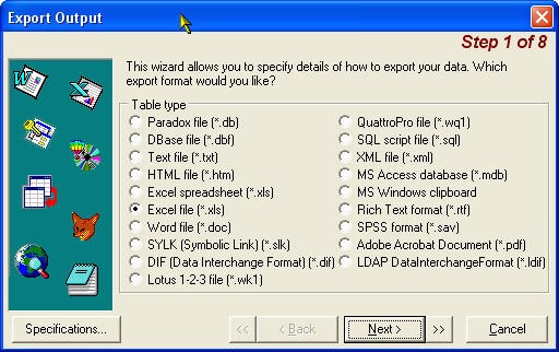
模型的输出可以导出的格式:
-
ASCII
-
Excel
-
Access
-
Rich text format
-
Adobe pdf
-
Lotus 123
-
Paradox
-
HTML
除了模型的计算结果外,导入的输出数据还可以显示在浓度对深度和浓度对时间图上。导入的数据可以来自模型,实验结果或理论结果。导入的数据可以从文件,项目中的模型中提取,也可以直接创建和输入。输入导入的数据后,可以对其进行编辑和删除。
系统要求
-
Windows 98 / NT / 2000 / XP或以上版本
-
64 MB的可用硬盘空间
-
128MB的RAM
-
CD或DVD驱动器
【英文介绍】
POLLUTE program provides fast, accurate, and comprehensive contaminant migration analysis capabilities. This program implements a one and a half dimensional solution to the advection-dispersion equation. Unlike finite element and finite difference formulations, POLLUTE does not require a time-marching procedure, and thus involves relatively little computational effort while also avoiding the numerical problems of alternate approaches.
With more then fifteen years utilization in industry, POLLUTE is a well tested contaminant migration analysis program which is widely used in landfill design and remediation. Landfill designs that can be considered range from simple systems on a natural clayey aquitard to composite liners, multiple barriers and multiple aquifers.
In addition to advective-dispersive transport, POLLUTE can consider
· non-linear sorption
· radioactive and biological decay
· transport through fractures
· passive sinks
· phase changes, and
· time-varying properties.
Feature Comparison
|
Feature |
Professional |
Standard |
|
Wizards and pre-created models |
Yes |
Yes |
|
Unlimited number of models |
Yes |
Yes |
|
Up to 200 layers |
Yes |
Yes |
|
Constant concentration boundary conditions |
Yes |
Yes |
|
Finite mass boundary condition |
Yes |
Yes |
|
Fixed outflow boundary condition |
Yes |
Yes |
|
Passive Sinks |
Yes |
Yes |
|
Linear sorption |
Yes |
Yes |
|
Non-linear sorption |
Yes |
No |
|
Fractures in layers |
Yes |
No |
|
Radioactive and biological decay |
Yes |
No |
|
Initial concentration profile |
Yes |
No |
|
Time-varying properties |
Yes |
No |
|
Monte Carlo Simulation |
Yes |
Yes |
|
Sensitivity Analysis |
Yes |
Yes |
POLLUTE Data Entry
Using the main menu bar at the of the screen, datasets can be created, edited, and executed. The output from these datasets can then be displayed and printed.
POLLUTE Deposit Data
Datasets can be created or edited using the Data Menu. A dataset consists of general deposit data, layer data, boundary conditions, and optional special features.
First, general data is entered about the model, such as:
· Title of the Dataset
· Number of Soil Layers (each layer can have different properties)
· Darcy Velocity through the soil layers
· Laplace Transform Parameters (defaults are usually sufficient)
POLLUTE Layer Data
For each layer, the following may be specified:
· Number of Sublayers
· Thickness
· Dry Density
· Coefficient of Hydrodynamic Dispersion
· Distribution Coefficient
· Type of Fractures (if present)
Any or all of the layers may be fractured. These fractures may be one, two, or three dimensional. In a fractured layer, the program considers advective-dispersive transport along the fractures coupled with diffusion into the matrix on either side of the fracture

POLLUTE Boundary Conditions
There are two boundaries for each dataset, one at the and one at the bottom of the layers. The boundary is usually the point of contact with the contaminant source (finite mass or constant concentration), and the bottom boundary is usually the point of contact with an aquifer (fixed outflow) or bedrock (zero flux).
Finite Mass Boundary Condition
The finite mass boundary condition may be used to represent contaminant sources such as landfills. Where the mass of contaminant is finite, the concentration of contaminant at the source will decline as contaminant mass is transported into the layers below or is removed by a leachate collection system.
Fixed Outflow Velocity Boundary Condition
This boundary condition may be used to represent an aquifer below the layers in the dataset. The concentration in this aquifer will vary with time as mass is transported into the aquifer from the layers above and is then transported away by the horizontal velocity in the base strata.
POLLUTE Special Features
In addition to the basic data parameters, many special features can also be used in the model. One or more of these special features may be selected from the multiple choice menu.
Radioactive/Biological Decay
Radioactive or biological decay can be modeled. First-order decay is considered by specifying the half lives for the source, layers, and base aquifer. The layers may have the same half-life, or the half-life can be specified as a function of depth.
Depth Interval Concentration Profile
To model background concentration in the layers, an initial concentration profile may be used. Using this option, the initial concentration in the layers can be specified as a function of depth. In addition, the flux into the soil and the base can be specified at the start time of the model.
Freundlich and Langmuir Nonlinear Sorption
Either Freundlich or Langmuir nonlinear sorption may be considered. When nonlinear sorption is used, the program splits the layers into sublayers and uses an iterative technique to determine the equivalent linear distribution coefficient for each sublayer.
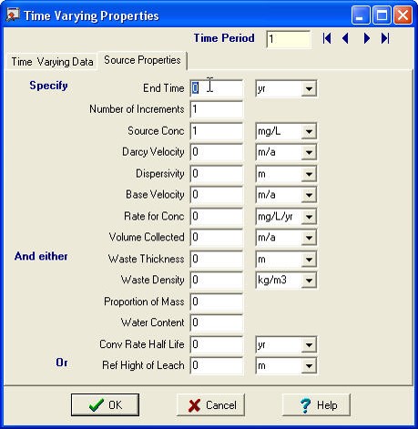
Properties Increment Within Groups
This option is used to vary properties of the model with time. The user may vary the source concentration, contaminant mass, volume of leachate collected, Darcy velocity, dispersivity and aquifer velocity. For example, this option can be used to simulate the progressive failure of the leachate collection system in a landfill. Time is divided into groups. In each group the properties may be constant with time or may increment linearly with time. The concentration in the source at the beginning of each time group may be specified or the concentration at the end of the last group may be used.
Passive Sink
One or more passive sinks may be used in the model. A passive sink is a layer where there is a horizontal velocity. This will have the effect of removing contaminants. Typically, a passive sink is used to represent secondary leachate collection systems or multiple aquifers.
Monte Carlo Variable Entry
Monte Carlo simulation may be used to evaluate the effects of uncertainty in the values of some of the model data. Using this approach, the uncertain data values are described using a probability distribution. After numerous simulations, a probability distribution is generated for the peak concentration of the contaminant at any depth.
Primary Liner (Subtitle D) Landfill
There are options to create and customize predefined models quickly and easily. These models include landfills with primary leachate collection and composite liners (Subtitle D).
Primary and Secondary Liner Landfill
There are options to create and customize predefined models quickly and easily. These models include landfills with primary leachate collection and composite liners (Subtitle D) and landfills with primary and secondary leachate collection and composite liners (Subtitle C). In these quick landfill entry options, layers such as the geomembrane, clay liner, aquitard, and aquifer can be included or discarded simply by the selecting Yes or No beside the layer name.
Leakage Rate (Subtitle D) Landfill
The leakage rate through the composite liner may be calculated using the method proposed by Giroud et al., 1992, and Giroud and Bonaparte, 1989. These calculations consider leakage due to permeation and defects in the geomembrane.
Geomembrane Hole Data
In addition to the type of contact between the geomembrane and the clay liner, the leakage will also depend on the type, size, and frequency of the defects.
Finite Mass Source
The landfill contaminant source can be either finite mass or constant concentration. If the source type is finite mass, the waste thickness and density, infiltration through the cover, and percentage of mass can be specified for the contaminant.
Primary Clay Liner or GCL
For each layer present in the model, the parameters may be specified in any units; the program will automatically convert all units to either SI or US. The liner can be either clay or a geosynthetic clay liner.
Aquifer
If an aquifer is present beneath the landfill, the thickness and porosity of the aquifer can be specified. The program will automatically calculate the minimum outflow velocity in the aquifer. This value or a higher value can be specified.
POLLUTE Model Execution
Calculate Concentrations
After the dataset has been created, the model can be executed. The concentration of the contaminant can be calculated at any number of specific depths or the maximum concentration can be determined automatically at any selected depth. Unlike other techniques that may take hours or days to prepare and execute models, the finite-layer technique is very quick. It typically takes only minutes to prepare and execute a model making it ideal for examining design alternatives and for sensitivity analysis.
POLLUTE Result Output
After the model has been executed, the output file can be displayed, graphed, and printed. Graphs can be concentration versus time, concentration versus depth, flux versus time, and color concentration. All of these graphs can also be easily printed on several types of printers. Default values for the graphs are automatically determined. These values can be easily changed to allow complete customization of the graph. For the concentration versus time graph, one or all of the depths may be plotted; likewise for time in the concentration versus depth graph.
Concentration Versus Time
Concentration with time graphs show the variation in the calculated concentration of the contaminant with time for the depths studied. Using these graphs, the peak concentration at a specific depth can be easily identified. This value is also automatically displayed at the of the graph.
Concentration Versus Depth
Concentration versus depth graphs show the change in contaminant concentration with depth, either for a specific time or for all the times that were calculated.
Flux Versus Time
The total flux into the of the soil layers and out of the bottom of the soil layers with time can be graphed.
Color Concentration Plot
The change in concentration with time and depth graph can be used to illustrate the movement of the contaminant plume into deeper depths over time.
Print Options
Graphs can be printed by pressing 'P' while they are displayed. Many of the features of the printed graph can be controlled such as the size, titles and fonts.
POLLUTE Tools
Tools are available to aid in creating and checking datasets.
Calculator
These tools include a calculator that can be used to determine Darcy velocity and contaminant mass.
Help
Context-sensitive help can be accessed any time by pressing the F1 key. The information displayed contains many cross-references which can be displayed by clicking on the highlighted text.
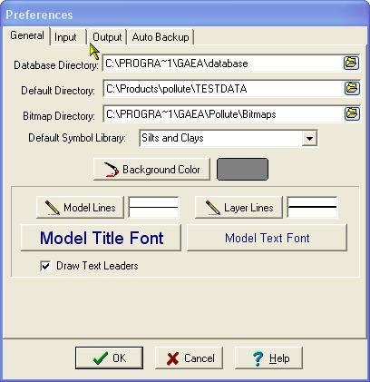
POLLUTE Preferences
The display colors, mouse buttons, and program environment can all be adjusted as desired. Many of the program features can be customized such as directories, file extensions, screen display type, and printer type.
Most popular screen types are supported, including Super VGA, VGA, and EGA, or the screen type can be automatically detected.
A large variety of printers are also supported such as Epson 9 and 24 pin, HP LaserJet, HP Pen Plotters, HP Paint Jet, and Postscript. Graphs can also be converted into PCX file format.


- 2026-06-22
- 2026-06-22
- 2026-06-18
- 2026-06-12
- 2026-06-12
- 2026-06-12

- 2026-06-22
- 2026-06-22
- 2026-06-22
- 2026-06-11
- 2026-06-11
- 2026-06-11